Previous
Machine Learning - Train/Test
Evaluate Your Model
In machine learning we create models to predict the outcome of certain events, such as in the previous chapter where we predicted the car's CO2 emissions while knowing the weight and size of the engine.
To measure whether the model is good enough, we can use a method called Train / Test.
What is Train/Test
Train / Test is a way to measure the accuracy of your model.
It is called Train / Test because it divides data set into two sets: training set and test set.
80% training, and 20% test.
You train a model using a training set.
You test the model using a test set.
Train a model means to create a model.
Test model means check the accuracy of the model.
Start With a Data Set
Start with a set of data you want to test.
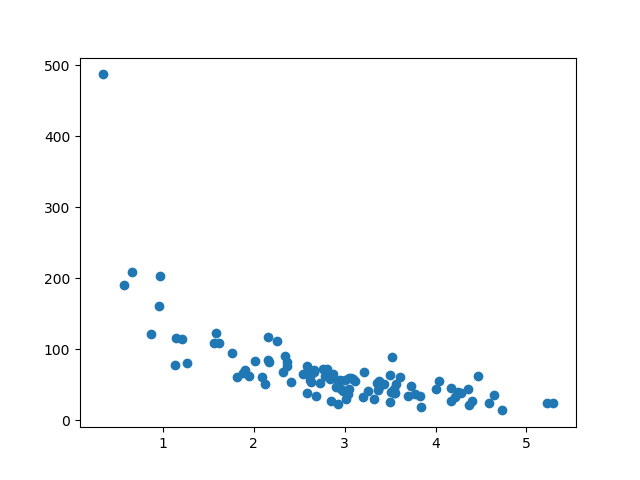
Our data set shows 100 customers in the store, as well as their shopping habits.
Example
import numpy
import matplotlib.pyplot as plt
numpy.random.seed(2)
x = numpy.random.normal(3, 1, 100)
y = numpy.random.normal(150, 40,
100) / x
plt.scatter(x, y)
plt.show()
Result
The x axis represents the number of minutes before making a purchase.
The y axis represents the amount of money spent on the purchase.
Split Into Train/Test
The training set should be a random selection of 80% of the original data.
The testing set should be the remaining 20%.
train_x = x[:80]

            train_y = y[:80]


            test_x = x[80:]

            test_y = y[80:]
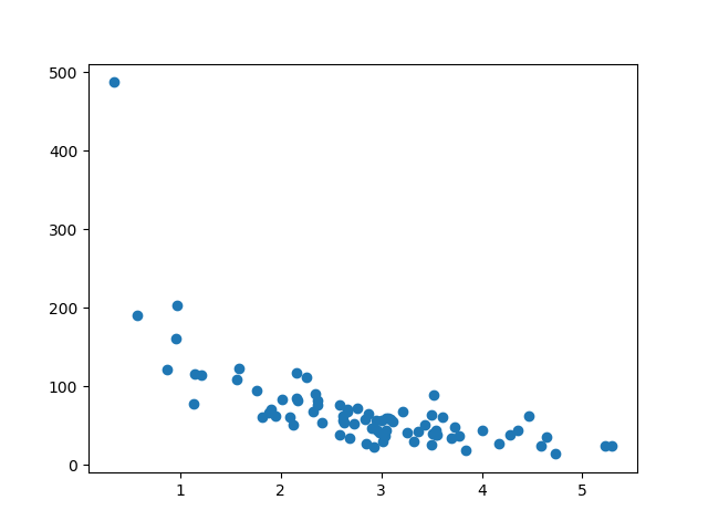
Display the Training Set
Display the scatter structure similar to the training set:
Example
plt.scatter(train_x,
train_y)
plt.show()
Result
It looks like the original data set, so it seems to be a fair selection:
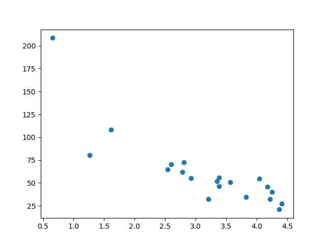
Display the Testing Set
To make sure the test set is not completely different, we will also look at the test set.
Example
plt.scatter(test_x,
test_y)
plt.show()
Result
The testing set also looks like the original data set:
Fit the Data Set
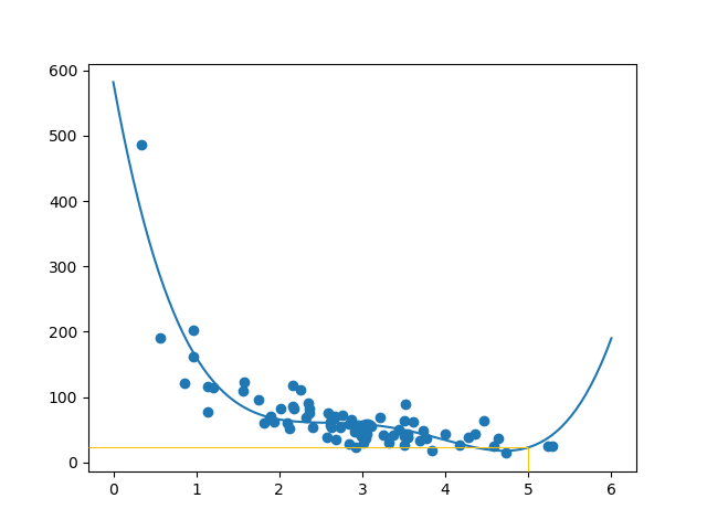
What does a data set look like? In my opinion I think a good equation would be a polynomial retreat, so let's draw a line of polynomial retreat.
To draw a line in the data points, we use the plot() method of the matplotlib module:
Example
import numpy
import
matplotlib.pyplot as plt
numpy.random.seed(2)
x =
numpy.random.normal(3, 1, 100)
y = numpy.random.normal(150, 40, 100) / x
train_x = x[:80]
train_y = y[:80]
test_x = x[80:]
test_y =
y[80:]
mymodel = numpy.poly1d(numpy.polyfit(train_x, train_y, 4))
myline = numpy.linspace(0, 6, 100)
plt.scatter(train_x, train_y)
plt.plot(myline, mymodel(myline))
plt.show()
Result

The result may support my suggestion for data equal to polynomial retrieval, although it may give us odd results if we try to predict values outside the data set. Example: the line shows that a customer who spends 6 minutes in a store will buy at a price of 200. That is a sign of overcrowding.
But what about double schooling? The R-square is a good indication of how well my data fits with the model.
R2
Do you remember R2, also known as R-squared?
It measures the relationship between the x-axis and the x-axis, and the value ranges from 0 to 1, where 0 means no relationship, and 1 means absolute correlation.
The sklearn module has a method called r2_score() that will help us find this relationship.
In this case we would like to measure the relationship between the minutes a customer stays in the store and how much they spend.
Example
How well does my training data fit in a polynomial regression?
import numpy
from sklearn.metrics import r2_score
numpy.random.seed(2)
x = numpy.random.normal(3, 1, 100)
y = numpy.random.normal(150, 40,
100) / x
train_x = x[:80]
train_y = y[:80]
test_x = x[80:]
test_y = y[80:]
mymodel = numpy.poly1d(numpy.polyfit(train_x, train_y,
4))
r2 = r2_score(train_y, mymodel(train_x))
print(r2)
Note: Result 0.799 indicates that OK relationship exists.
Bring in the Testing Set
Now we have created the right model, at least when it comes to training.
Now we want to test the model with test data again, to see if it gives us the same result.
Example
Let us find the R2 score when using testing data:
import numpy
from sklearn.metrics import r2_score
numpy.random.seed(2)
x = numpy.random.normal(3, 1, 100)
y = numpy.random.normal(150, 40,
100) / x
train_x = x[:80]
train_y = y[:80]
test_x = x[80:]
test_y = y[80:]
mymodel = numpy.poly1d(numpy.polyfit(train_x, train_y,
4))
r2 = r2_score(test_y, mymodel(test_x))
print(r2)
Note: The result of 0.809 indicates that the model is equal to the test set, and we are confident that we can use the model to predict future values.
Predict Values
Now that we have found out that our model is OK, we can start predicting new values.
Example
How much money will a buying customer spend, if she or he stays in the shop for 5 minutes?
print(mymodel(5))
The model predicted that the customer would spend $ 22.88, as seen in the diagram: